Optimal stopping with a deck of cards

In the midst of this calamitous year I was lucky to find some respite in the following classic problem, posed in a random Slack channel at work:

A standard deck of cards with \(m=26\) black and red cards each is shuffled perfectly, and you are offered a game where you may draw cards one at a time without replacement until you choose to stop, or no more cards remain. Each black card drawn earns you $1, whereas each red card drawn loses you $1.

What is the value of this game, played optimally? What about in the limit as \(m\rightarrow\infty\)?

An empirical result

First, let’s try to compute some empirical results for fixed, finite \(m\).

Letting the game value with \(b>0\) black cards and \(r>0\) red cards left in the deck be \(V(b, r)\), we note that choosing to stop yields the immediate payoff of \(m - b - (m - r) = r - b\), and choosing to draw yields a black card and payoff \(V(b-1, r)\) with probability \(\frac{b}{b+r}\) and a red card and payoff \(V(b, r-1)\) with probability \(\frac{r}{b+r}\). The game value \(V(b, r)\) is thus the maximum of these two choices. We may also note \(V(0, r) = r\) since we cannot improve by drawing; also \(V(b, 0)=0\) since we may always improve to 0 by drawing out the deck.

A bit of Python code computes the game value \(V(26, 26)\):

memo = {}
def value(black, red):
    if black == 0:
        return red
    if red == 0:
        return 0
    return memo[(black, red)] if (black, red) in memo else memo.setdefault(
        (black, red), max(
            red - black,
            (black / (black + red) * value(black - 1, red)
            + red / (black + red) * value(black, red - 1)))
    )
print(value(26, 26))  # 2.6244755489939244

From the above recursion, it’s clear that \(V(m, m)\) is actually rational. For instance, I found an OEIS entry which gives the first 26 values - turns out the precise value of \(V(26, 26)\) is \(\frac{41984711742427}{15997372030584}\) - I’d be interested in knowing whether there’s a general analytical formula!

A conjecture for the limit

To investigate the limit as \(m\rightarrow\infty\), we can use the routine above to generate some data:

import numpy as np
import matplotlib.pyplot as plt
x = np.arange(1, 1000)
y = np.array([value(x_, x_) for x_ in x])
fig, ax = plt.subplots(1, 2, figsize=(20, 4))
ax[0].plot(x, y)
ax[1].plot(np.log(x), np.log(y))

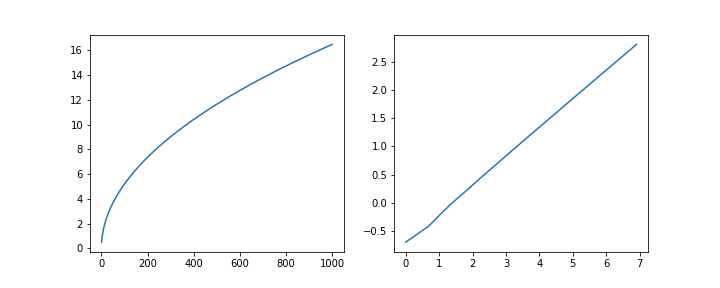
The log-log plot is pretty close to linear with slope approaching what looks to be \(\frac{1}{2}\):

((ln_y[:-1] - ln_y[1:]) / (ln_x[:-1] - ln_x[1:]))[-5:]
# array([0.50080497, 0.50080423, 0.50080348, 0.50080275, 0.50080202])

and intercept roughly:

np.exp(ln_y[-1] - ln_x[-1] * (ln_y[-1] - ln_y[-2]) / (ln_x[-1] - ln_x[-2]))
# 0.518562756949232

so that we may guess that in the limit:

$\lim_{m\rightarrow\infty}\frac{V(m, m)}{\sqrt{m}} = V \approx 0.52$

A sketched proof

As it turns out, the mathematics involved in this problem are pretty well known - for instance, they were worked out explicitly by the late Professor Larry Shepp in 1969¹. In this post, I’ll share my notes while trying to follow along!

The Brownian Bridge

First, we must invoke the stochastic process known as the Brownian Bridge, which is loosely the standard Wiener process “tied down” to be 0 at both \(t=0\) and \(t=1\). That is, with \(W(t), t\geq0\) the standard Wiener process with independent normal increments \(W(t) - W(s) \sim \mathcal{N}(0, t-s)\), define the standard Brownian Bridge \(B(t), t\in[0, 1]\) to be the unique Gaussian process with mean \(\mathop{\mathbf{E}}B(t) = 0\) and covariance \(\mathbf{Cov}[B(s),B(t)] = s(1- t)\) for \(s \leq t\).

As it turns out, in the limit, our process \(S_i^{(m)}, i\in(0, 1, 2, \dots, 2m)\) of total current winnings after drawing \(i\) cards through a deck of \(2m\) cards, is just a time and space scaled Brownian Bridge, in the sense:

$X^{(m)}(t):=\frac{1}{\sqrt{2m}}S_{\lfloor{2mt}\rfloor}^{(m)} \xrightarrow{\mathcal{D}} B(t)$

To see this informally, note that: \(S_i^{(m)} = \sum_{a=1}^i \xi_a\) where each \(\xi_a\) for \(a\in(1, 2, \dots, 2m)\) represents the draw of the \(a\)-th card - i.e. they are identically (but not independently) distributed with \(\mathbf{P}(\xi_a=1)=\mathbf{P}(\xi_a=-1)=\frac{1}{2}\), so that \(\mathop{\mathbf{E}}\xi_a=0\), \(\mathop{\mathbf{Var}}\xi_a=1\), and for \(a\neq b\):

$\mathbf{Cov}[\xi_a,\xi_b]=\mathop{\mathbf{E}}\xi_a\xi_b=\frac{n-1}{2n-1}-\frac{n}{2n-1}=-\frac{1}{2n-1}$

So by linearity of expectation we immediately have:

$\mathop{\mathbf{E}}S_{i}^{(m)} = \frac{1}{\sqrt{2m}}\mathop{\mathbf{E}}\sum_{a=1}^{i}\xi_a=\frac{1}{\sqrt{2m}}\sum_{i=1}^{i}\mathop{\mathbf{E}}\xi_a=0$

As for the covariance, letting \(s\leq t\) without loss of generality:

$\begin{aligned} \mathbf{Cov}\left[X^{(m)}(s),X^{(m)}(t)\right] & =\frac{1}{2m}\mathop{\mathbf{E}}\sum_{a=1}^{\lfloor 2ms\rfloor}\xi_a\sum_{b=1}^{\lfloor 2mt\rfloor} \xi_b \\ & = \frac{1}{2m}\left(\lfloor 2ms\rfloor(1)-\lfloor 2ms\rfloor(\lfloor 2mt\rfloor-1)\frac{1}{2m-1}\right) \\ & = \frac{\lfloor 2ms\rfloor}{2m}\left(1-\frac{\lfloor 2mt\rfloor-1}{2m-1}\right) \\ & \rightarrow s(1-t) \end{aligned}$

However, it remains to be shown that limiting process is Gaussian, perhaps using some suitable central limit theorem. I haven’t managed to find one that works, and of course, this might not even follow!

More formally, I think one can demonstrate the equivalence to a Brownian Bridge by noting that our process \(S_i^{(m)}\) has the same distribution as a simple random walk over \(\mathcal{Z}^1\), conditioned to be \(0\) at \(2m\); from there, Donsker’s invariance principle can be applied to show that the rescaled random walk converges in law to Brownian motion.

The optimal stopping time

We will now follow along with Shepp’s proof in Sections 1, 2, 3, and 6 of ¹, which goes roughly as follows:

With \(W(t)\) a standard Wiener process, and fixed real constants \(u, b\) with \(-\infty < u < \infty, b > 0\), let \(T\) range over all possible stopping times for this process (i.e. strategies to choose a time \(t \geq 0\) that is non-anticipating²) and consider the new (seemingly arbitrary) objective:

$\tilde{V}(u, b) = \sup_{T}\mathbf{E} \left[\frac{u + W(T)} {b + T}\right]$

We will see eventually how this connects back to the Brownian Bridge.

Now notice the “scale-change invariance property” of \(W(t)\), whereby \(\dfrac{W(bt)}{\sqrt{b}}\) is again a standard Wiener process for any \(b>0\)! This yields:

$\mathbf{E} \left[\frac{u + W(t)} {b + t}\right] = \frac{1}{\sqrt{b}} \mathbf{E} \left[\frac{\frac{u}{\sqrt{b}} + \frac{W(b\frac{t}{b})}{\sqrt{b}}} {1 + \frac{t}{b}}\right] = \frac{1}{\sqrt{b}} \mathbf{E} \left[\frac{\frac{u}{\sqrt{b}} + W^*(t^*)} {1 + t^*}\right]$

where \(t^* = \frac{t}{b}\) is a non-anticipating stopping time for \(W^*(t) = \dfrac{W(bt)}{\sqrt{b}}\). Now taking the supremum over all \(T\), we obtain:

$\tag{1} \tilde{V}(u, b) = \frac{1}{\sqrt{b}}\tilde{V}(\frac{u}{\sqrt{b}}, 1)$

Now, clearly \(\tilde{V}(u, 1) \geq u\) by considering the deterministic stopping time \(T=0\). Intuitively, the larger \(u\) is, the more difficult it is to beat this, as \(\frac{u + W(t)} {1 + t} - u = \frac{W(t) - ut} {1 + t}\); thus \(\tilde{V}(u, 1) = u\) when \(u \geq \gamma\) for some \(\gamma > 0\), associated with the optimal stopping time \(T=0\), i.e. deterministically stopping immediately. It follows from (1) that stopping at \(0\) is also optimal for general \(b\) and the same \(\gamma\) when \(u \geq \gamma \sqrt{b}\), in which case we then have \(\tilde{V}(u, b) = \frac{u}{b}\).

When \(u < \gamma \sqrt{b}\), since the Wiener process is memoryless, intuitively the optimal stopping rule for any \(u, b\) is to stop the first time \(\tau\) that \(u + W(\tau) \geq \gamma\sqrt{b + \tau}\), because at this time, “restarting” the Wiener process with \(u’ = u + W(\tau)\) and \(b’ = b + \tau\) gives the criteria we have determined above.

Generalize for any \(c>0\) the stopping time \(\tau_c = \min \{ t: u + W(t) \geq c\sqrt{b + t} \}\). (The optimal stopping time we determined above is then a specific instance, \(\tau_\gamma\) for the still-unknown constant \(\gamma\)). Let \(f_c(t)\) be the density function for \(\tau_c\). It can be shown³ that:

$\int_0^\infty e^{\lambda c \sqrt{b + t} - \lambda u - \frac{\lambda^2 t}{2}} f_{c}(t) \mathop{}\!\mathrm{d}t = 1$

for \(\lambda>0\) and \(u < c \sqrt{b}\). From this we have:

$\begin{gathered} & \Rightarrow & \int_0^\infty \int_0^\infty c e^{\lambda c \sqrt{b + t} - \frac{\lambda^2 (b + t)}{2}} f_{c}(t) \mathop{}\!\mathrm{d}t \mathop{}\!\mathrm{d}\lambda & = & c \int_0^\infty e^{\lambda u - \frac{\lambda^2 b}{2}} \mathop{}\!\mathrm{d}\lambda \\ & \Rightarrow & \int_0^\infty \frac{c}{\sqrt{b + t}} f_{c}(t) \mathop{}\!\mathrm{d}t \int_0^\infty e^{c y - \frac{y^2}{2}} \mathop{}\!\mathrm{d}y & = & c \int_0^\infty e^{\lambda u - \frac{\lambda^2 b}{2}} \mathop{}\!\mathrm{d}\lambda \\ & \Rightarrow & \mathbf{E} \left[ \frac{c}{\sqrt{b + \tau_c}} \right] & = & c \int_0^\infty e^{\lambda u - \frac{\lambda^2 b}{2}} \mathop{}\!\mathrm{d}\lambda \left( \int_0^\infty e^{c y - \frac{y^2}{2}} \mathop{}\!\mathrm{d}y \right)^{-1} \\ & \Rightarrow & \mathbf{E} \left[\frac{u + W(\tau_c)} {b + \tau_c}\right] & = & c \int_0^\infty e^{\lambda u - \frac{\lambda^2 b}{2}} \mathop{}\!\mathrm{d}\lambda \left( \int_0^\infty e^{c y - \frac{y^2}{2}} \mathop{}\!\mathrm{d}y \right)^{-1}\\ \end{gathered}$

where on the first line we have multiplied through by \(c e^{\lambda u - \frac{\lambda^2 b}{2}}\), integrated over \(\lambda\), and interchanged integrals; on the second line we have made the change of variables \(\lambda\sqrt{b + t} = y\) on the LHS, and split the independent integrals; on the third line we apply the “law of the unconscious statistician”; and on the fourth we note that by the definition of \(\tau_c\) we have precisely: \(u + W(\tau_c) = c\sqrt{b + \tau_c}\).

In this last equality, the LHS is precisely the expected payoff for \(\tau_c\) whose supremum is \(\tilde{V}(u, b)\). And, incredibly, though the RHS depends on \(c, u, b\); its maximum along \(c\) for fixed \(u, b\) is independent of \(u, b\)! This is the value \(\gamma\) and with a bit of calculus (omitted for now) it can be shown that \(\gamma\) is the unique real solution to:

$\gamma = (1-\gamma)^2 \int_0^\infty e^{\lambda \gamma - \frac{\lambda^2}{2}} \mathop{}\!\mathrm{d}\lambda$

which is about \(0.8399\):

lo, hi, y = 0.0, 1.0, 1.0
while abs(y) > 1e-9:
    c = (lo + hi) / 2
    y = (1 - c**2) * integrate.quad(lambda z: np.exp(z*c - z**2 / 2), 0, np.inf)[0] - c
    if y > 0:
        lo = c
    else:
        hi = c
print(c)  # 0.8399236756922619

We are almost done. To connect back to the Brownian Bridge \(B(t)\), recall we were originally interested in (as the limit of the discrete card-drawing process):

$V = \sqrt{2} \sup_{T}\mathbf{E} B(T)$

where now \(T\) is a non-anticipating stopping time \(0 \leq T \leq 1\), and the extra factor \(\sqrt{2}\) arises from the fact that the discrete card-drawing process is normalized by \(\sqrt{2m}\), not \(\sqrt{m}\), in the passage to the limit.

Note that the Brownian Bridge has the representation \(B(t) = (1 - t)W(\frac{t}{1 - t})\), and make the change of variable \(t’ = \frac{t}{1-t}\), from which we see:

$V = \sqrt{2} \sup_{T'}\mathbf{E} \frac{1}{1 + T'}W(T') = \sqrt{2} \tilde{V}(0, 1)$

Putting everything together:

$\begin{aligned} V = \sqrt{2} \tilde{V}(0, 1) & = \sqrt{2} \gamma \left( \int_0^\infty e^{-\frac{\lambda^2}{2}} \mathop{}\!\mathrm{d}\lambda \right) \left( \int_0^\infty e^{c y - \frac{y^2}{2}} \mathop{}\!\mathrm{d}y \right)^{-1} \\ & = \sqrt{2} (1 - \gamma^2) \left( \int_0^\infty e^{-\frac{\lambda^2}{2}} \mathop{}\!\mathrm{d}\lambda \right) \\ & = \sqrt{2} (1 - \gamma^2) \sqrt{ \frac{\pi}{2} } \\ & \approx 0.522 \end{aligned}$

Pretty neat!

1. Shepp, L. A. Explicit Solutions to Some Problems of Optimal Stopping. Ann. Math. Statist. 40 (1969), no. 3, 993–1010. ↩ ↩²

2. More rigorously, we could say \(T\) is a stopping-time with respect to the filtration generated by the Wiener process; that is, the event \({T \leq t} \in \mathcal{F}_{t}\) for all \(t\geq 0\). ↩

3. A detailed proof is found in Sections 2 & 3 of ¹. As Shepp mentions, the proof is similar to that of Wald’s “fundamental identity”, which can be found in Section 3 here. ↩